Explorative analysis

First, we download the data from the Strava-API:

# Config
client_id <- 38395
secret <- keyring::key_get("secret", "strava")
app_name <- "Bloggdata"

# Get token and get data (this part is commented out to save time, read in RDS instead)
# stoken <- httr::config(token = strava_oauth(app_name, client_id, secret, app_scope="activity:read_all"))
# my_acts <- get_activity_list(stoken)
# 
# df <- compile_activities(my_acts)
# saveRDS(df, file = here::here("./content/post/strava_df.rds"))
df <- readRDS(here::here("./content/post/strava_df.rds"))

Since we are interested in number of kudos, private rides should be filtered:

df <- df %>% 
  filter(visibility == "everyone")

Let’s look at my unimpressive distribution of kudos:

df %>% 
  ggplot(aes(x = kudos_count)) +
  geom_histogram(aes(y = ..density..), bins = 20, color = "black", fill = "grey") +
  geom_density(fill = "steelblue", alpha = 0.5)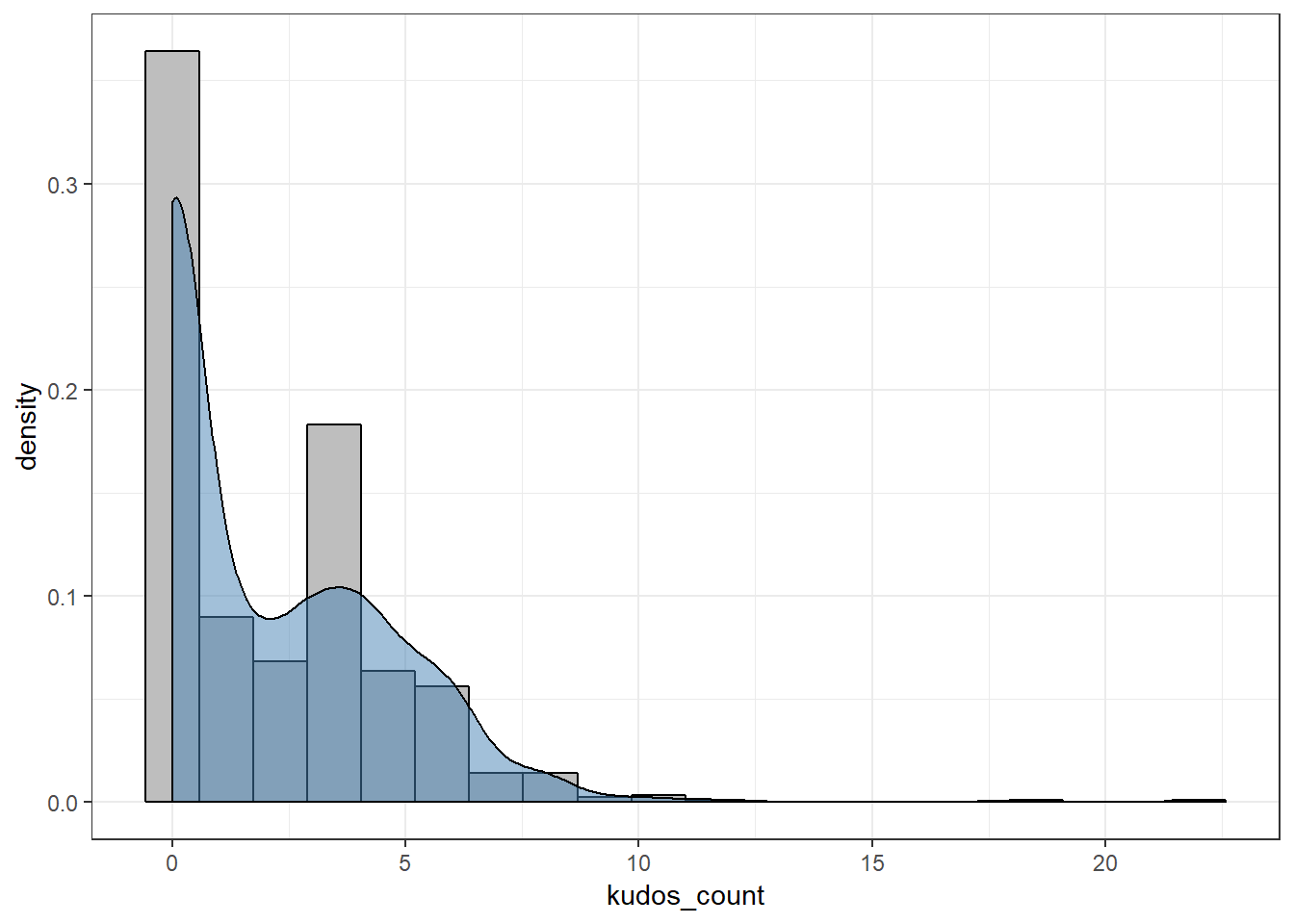

We see that we are dealing with what looks like a zero-inflated distribution. This indicates that we should probably have used a zero-inflated Poisson model, which means that two models are created simultaneously: a logistic regression to estimate the probability of getting 0 or more kudos, and a Poisson model to estimate the number of kudos.

However, I stick with a normal Poisson-model for simplicity of interpretation, moreover, the zero-inflated approach requires more data to work well.

We should also investigate how the number of kudos depends on the date of the activity:

df %>% 
  ggplot(aes(x = as_date(start_date), y = kudos_count)) +
  geom_jitter(alpha = 0.5) +
  geom_smooth() +
  labs(x = "date")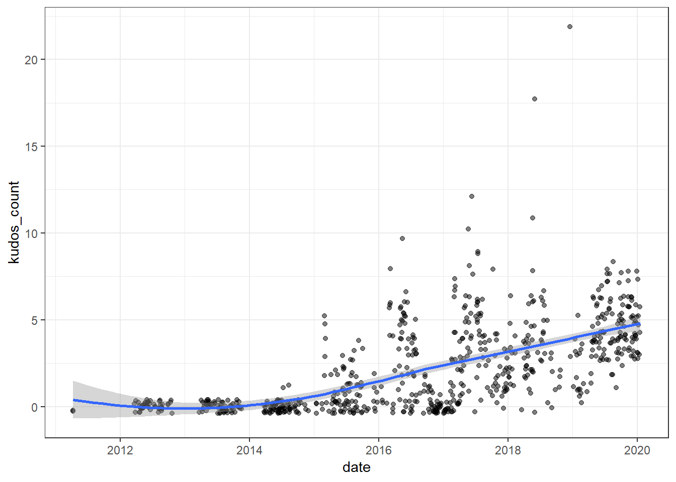

We see that we have a positive trend, so we have to account for this when modelling in order to isolate the effects of other relevant variables. Based on the observed trend, it appears sufficient to use a simple linear, year-wise trend.

Preparing the data

First, let’s create a recipe in order to add some useful variables. Note that I don’t bother using the train/test-approach here, because I’m not really worried about the model’s ability to predict anything, I just want to analyze the causal relationships.

• step_date is used to get useful time-variables such as day of the week.
• step_unknown replaces NA with the string “unknown”. This is useful because glm automatically drops the entire row if one value is NA.
• step_meanimpute replaces rides with no suffer-score (e.g missing heart rate) with the average.
• step_other is useful for factor-variables where some factors have too few levels. Threshold = 10 ensures that only factor levels with more than 10 observations are kept.

rec <- recipe(kudos_count ~ ., data = df) %>%
  step_mutate(date = as_datetime(start_date_local),
              hour_started = as.numeric(hour(date)),
              suffer_score = as.numeric(suffer_score)) %>% 
  step_date(date) %>%
  step_unknown(location_city) %>%
  step_meanimpute(suffer_score) %>% 
  step_other(location_city, threshold = 10) %>%
  step_other(type, threshold = 10)

prep_rec <- prep(rec, training = df)
df_prepped <- bake(prep_rec, df)

# Make categories of time of day
df_prepped <- df_prepped %>% 
  mutate(time_of_day = case_when(hour_started > 18 ~ "evening",
                                 hour_started > 11 ~ "day",
                                 hour_started > 6 ~ "morning",
                                 TRUE ~ "night"))

Creating the model

Let’s create the model, using the glm-function from stats while specifying that we want a Poisson-model.

formula <- as.formula(kudos_count ~
                        + average_speed
                        + distance
                        + has_heartrate
                        + suffer_score
                        + total_elevation_gain
                        + location_city
                        + type
                        + total_photo_count
                        + date_dow
                        + date_month
                        + date_year
                        + time_of_day)

model <- glm(formula, data = df_prepped, family = "poisson")

I present the results using the DT-package, which allows the creation of HTML-tables. Rows with statistically significant results are colored in red using the “formatStyle”-function.

model_summary <- broom::tidy(model)
output_table <- model_summary %>%
  mutate_if(is.numeric, ~ round(.x, 2)) %>% 
  DT::datatable(rownames = FALSE) %>% 
  DT::formatStyle(
  'p.value',
  target = 'row',
  backgroundColor = DT::styleInterval(c(0.05, 0.1), c('red', 'pink', "white"))
)

# Note: this last line is only required for displaying the table on blogdown-websites.
widgetframe::frameWidget(output_table)

Causal analysis

Looking at the effects present in the model, we can make the following conclusions:

• Speed, distance and elevation are all quite significant, as one would expect. People are more likely to give you a kudos when they are impressed by your effort!
• Virtual rides get significantly fewer kudos. Clearly, no one are impressed by my long, sweaty indoor rides.
• Photos don’t matter. This one was a bit surprising to me. Maybe my photos are just terrible?
• Tuesday is the best day of the week for getting kudos, while Thursday is the worst (seems a bit random, but OK)
• May is the best month to upload rides, February is the worst.
• Time of day doesn’t appear to be very important. In fact, the factor level night is significant, but I am pretty sure this is spurious - all of my rides starting at night have been races, which are likely to receive more kudos. Since I haven’t controlled for whether a ride is a race or a training ride with any other variable, this is most likely the effect that’s picked up here.

Clearly, if you want to become popular on Strava, you should have a really long, fast and hilly ride on a Tuesday in May.

Disclaimer: Statistical results with n = 1 (myself) may not be representative of the general population. More studies, with slightly larger sample size, are required to make meaningful and generalizable causal inference…

Evidently, taking photos like this is a waste of time!