Analyzing Twitter-sentiments of the Tour de France favourites

Preparing the data

# Load packages
library(tidyverse)
library(tidytext)
library(rtweet)
library(wordcloud)
library(ggforce)
library(ggforce)

theme_set(theme_minimal())

We will use the “rtweets” package to access all available tweets concerning the two riders. If you wish to replicate the analysis, please note that you need to authenticate your Twitter-oath before downloading the data.

First, we specify the search words and collect the data in a data-frame. Note that Twitter only keeps data for up to 10 days, so I save the data as a .rds file in order to be able to replicate the analysis in the future.

# List of search-words to map over
searchWords <- c("egan bernal", "geraint thomas")

# Create data frame of tweets using purrr
df <- map_df(searchWords, ~ search_tweets(q = ., n = 10000, include_rts = FALSE), .id = "Rider")

# Note that retweets are excluded in order to get unique tweets

# Add variables
df <- df %>%
  mutate(Rider = if_else(Rider == 1, "Egan Bernal", "Geraint Thomas"),
         Date = lubridate::as_date(created_at))

# Save dataset so you can replicate the analysis - note that the Twitter API throws away data after 10 days
saveRDS(df, "tdf0307.rds")

We can start by looking at the number of tweets per day.

df %>%
  group_by(Rider, Date) %>%
  summarise(Number_of_tweets = n()) %>%
  ggplot(aes(x = Date, y = Number_of_tweets, color = Rider)) +
           geom_line() +
           geom_point() +
  labs(y = "Number of tweets") +
  geom_mark_ellipse(x = lubridate::ymd("2019-06-23"), y = 240, description = "Bernal wins TDS", inherit.aes = F, fill = "lightblue") +
  theme(legend.position="bottom")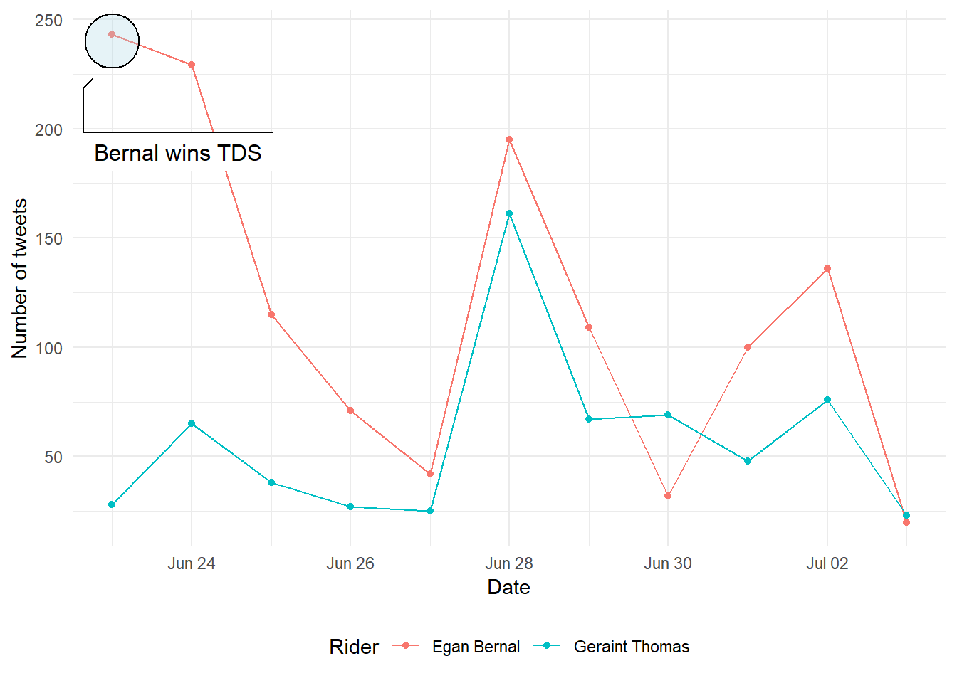

As one would expect, Egan Bernal was far more talked about towards the end of June, since he won the Tour de Suisse in this period. However, he’s also been slightly more popular on Twitter in the last couple of days - but the difference appears minimal.

Sentiment analysis

First, we will look at how the tweets of each rider can be mapped to different emotions such as anger, happiness and anticipation. This is done by using the “nrc”-database available through the excellent package Tidytext.

# Get the tokens per rider
tokens <- df %>% 
  group_by(Rider) %>%
  unnest_tokens(word, text)

# Access emotions through an inner-join with the sentiment-database
emotions <- tokens %>%
  inner_join(get_sentiments("nrc")) %>% 
  count(sentiment) %>%
  mutate(share_of_words = n/sum(n))

# Plot the results
ggplot(emotions, aes(x = sentiment, y = share_of_words, fill = Rider)) +
  geom_bar(stat = "identity", position = "dodge") +
  labs(y = "Share of tweets", x = NULL, title = "Twitter sentiment: Bernal vs Thomas") +
  theme_bw() +
  theme(legend.position="bottom")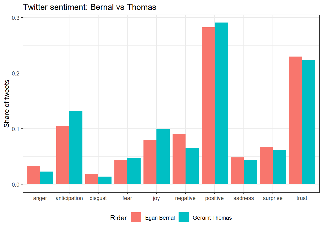

There are some small differences, such as the degree of “anticipation” being higher for Geraint Thomas, but the results hardly look statistically significant

However, the data set is probably too small to detect differences over so many possible emotions. Therefore, we can focus exclusively on classifying positive/negative emotions. For this simplification, we can use the “bing”-database.

Next, we can look at how these emotions have evolved over time.

tokens_trend <- df %>% 
  mutate(Date = as.Date(created_at)) %>%
  group_by(Rider, Date) %>%
  unnest_tokens(word, text)

sentiment_trend <- tokens_trend %>%
  inner_join(get_sentiments("bing")) %>% 
  count(sentiment) %>%
  mutate(share_of_tweets = n/sum(n))

# Plot the trend
sentiment_trend %>%
  filter(sentiment == "positive") %>%
  ggplot(aes(x = Date, y = share_of_tweets, color = Rider)) +
  geom_line(alpha = 0.5) +
  geom_point() +
  labs(y = "Share of positive words", title = "Trend in sentiment") +
  theme(legend.position="bottom")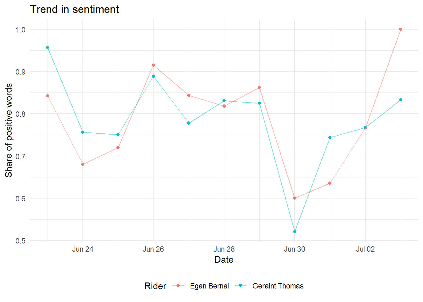

Again, there really aren’t any signs that one rider is more popular than the other.

Wordclouds

Finally, I will create word clouds to investigate the most common words used in tweets concerning each rider. First, we can look at the word cloud for Egan Bernal.

# Find words connected to emotions
emotions <- tokens %>%
  ungroup() %>%
  inner_join(get_sentiments("nrc"))

# Plot wordcloud
emotions %>%
  filter(Rider == "Egan Bernal") %>%
  anti_join(stop_words) %>%
  count(word) %>%
    with(wordcloud(words = word, freq = n, max.words = 100, min.freq = 5, random.order=FALSE, rot.per = 0.35, colors = brewer.pal(8, "Dark2")))

As we can see, the most prominent words are positively loaded words such as “team”, “champion”, “victory” and “winner”. Note that these words are heavily affected by the abundant amount of tweets on the day of his Tour de Suisse-victory. In addition, it seems like many people agree that he is quite unpredictable - which is often a prominent trait among younger riders.

Here is the corresponding plot for Geraint Thomas:

emotions %>%
  filter(Rider == "Geraint Thomas") %>%
  anti_join(stop_words) %>%
  count(word) %>%
  with(wordcloud(words = word, freq = n, max.words = 100, min.freq = 5, random.order=FALSE, rot.per = 0.35, colors = brewer.pal(8, "Dark2")))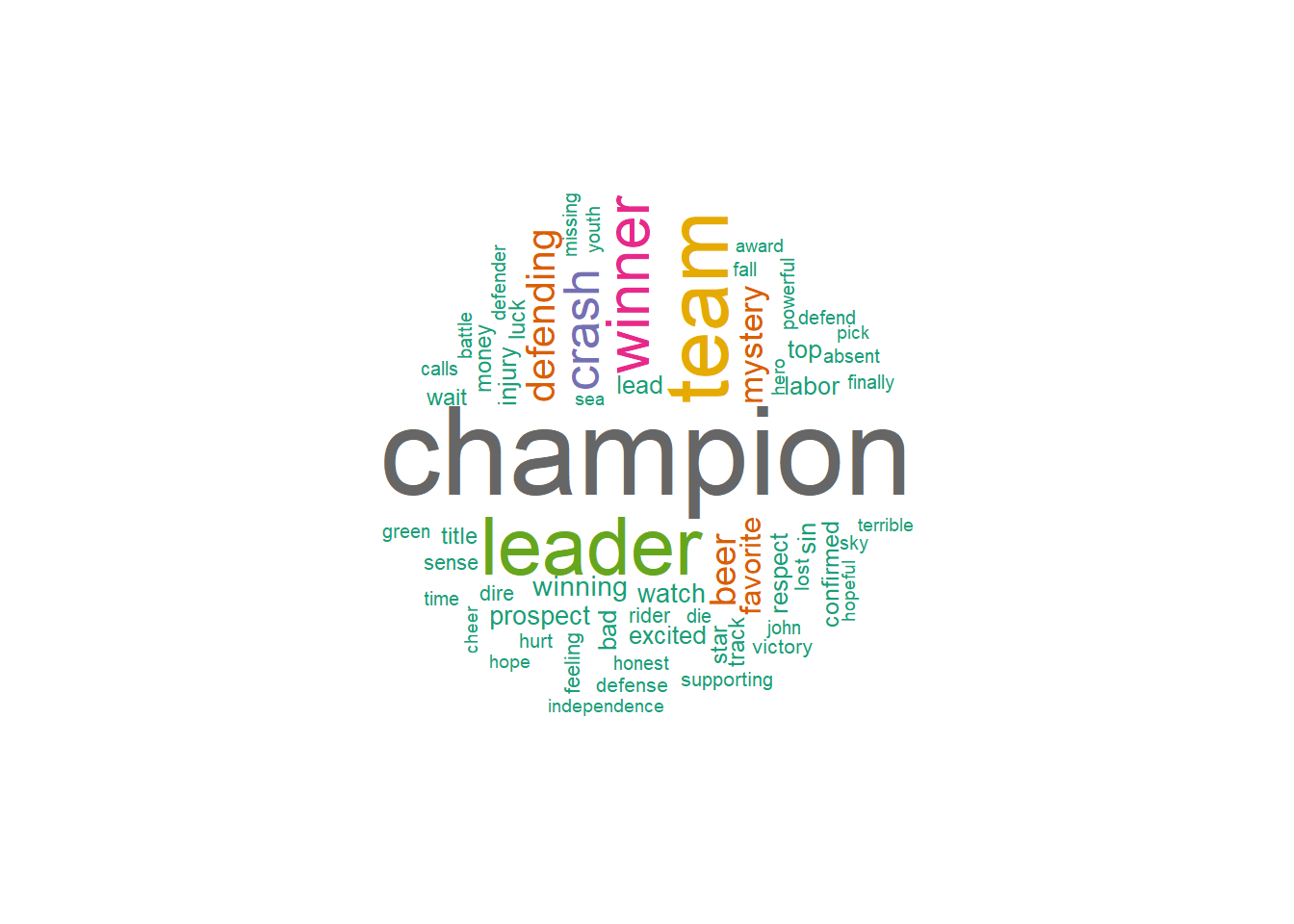

Final remarks

Obviously, this is not a very scientific exercise and one cannot expect to get a lot of insight from analyzing Twitter-data (it’s fun, though). There are lots of issues with this approach, such as:

• Tweets being written in different languages, i.e. tweets about Bernal are more likely to be in Spanish
• Other people with the same names could influence the results
• Sentiment analysis is in general quite unstable, particularly when applied on “internet slang”. I saw a really interesting talk about this at the eRum conference last year, which can be found here: https://www.youtube.com/watch?v=RT75_leoOSU&feature=youtu.be