In today’s blogpost I will look at historical data from the Tour de France. This data was used in the Tidytuesday series back in April, but I thought I’d take a closer look at it now as I currently suffer from Tour de France withdrawal symptoms (a July without Tour de France is like December without Christmas).
First, let’s load the data and have a look at the structure.
tdf <- tidytuesdayR::tt_load('2020-04-07')##
## Downloading file 1 of 3: `stage_data.csv`
## Downloading file 2 of 3: `tdf_stages.csv`
## Downloading file 3 of 3: `tdf_winners.csv`We have three different datasets, which we will call “rankings”, “stages” and “winners”.
rankings <- tdf$stage_data
stages <- tdf$tdf_stages
winners <- tdf$tdf_winners- The “rankings” data set contains info about the rankings of each stage per year, with some information about each rider such as age and bib number. Each row in the dataset is a rider’s placement on a given stage.
- The “stages” dataset contains more information about the stage, such as the distance, the type and the geographics.
- The “winners” dataset contains more information about the overall winner, such as the distance covered, time used and total number of stage wins.
Now we are ready to explore some statistics.
Number of stage wins over the years
winners %>%
  mutate(rolling_mean_5 = zoo::rollmean(stage_wins, 5, align = "right", fill = 0)) %>%
  ggplot(aes(x = year(start_date), y = stage_wins)) +
  geom_col(fill = "seagreen4", color = "seagreen4", alpha = .3) +
  geom_line(aes(y = rolling_mean_5), color = "blue", size = 0.9) +
  labs(y = "# of stage wins", x = "TDF-edition", title = "Development in number of stage wins per TDF-winner") +
  guides(color = guide_legend(override.aes = list(alpha = 1)))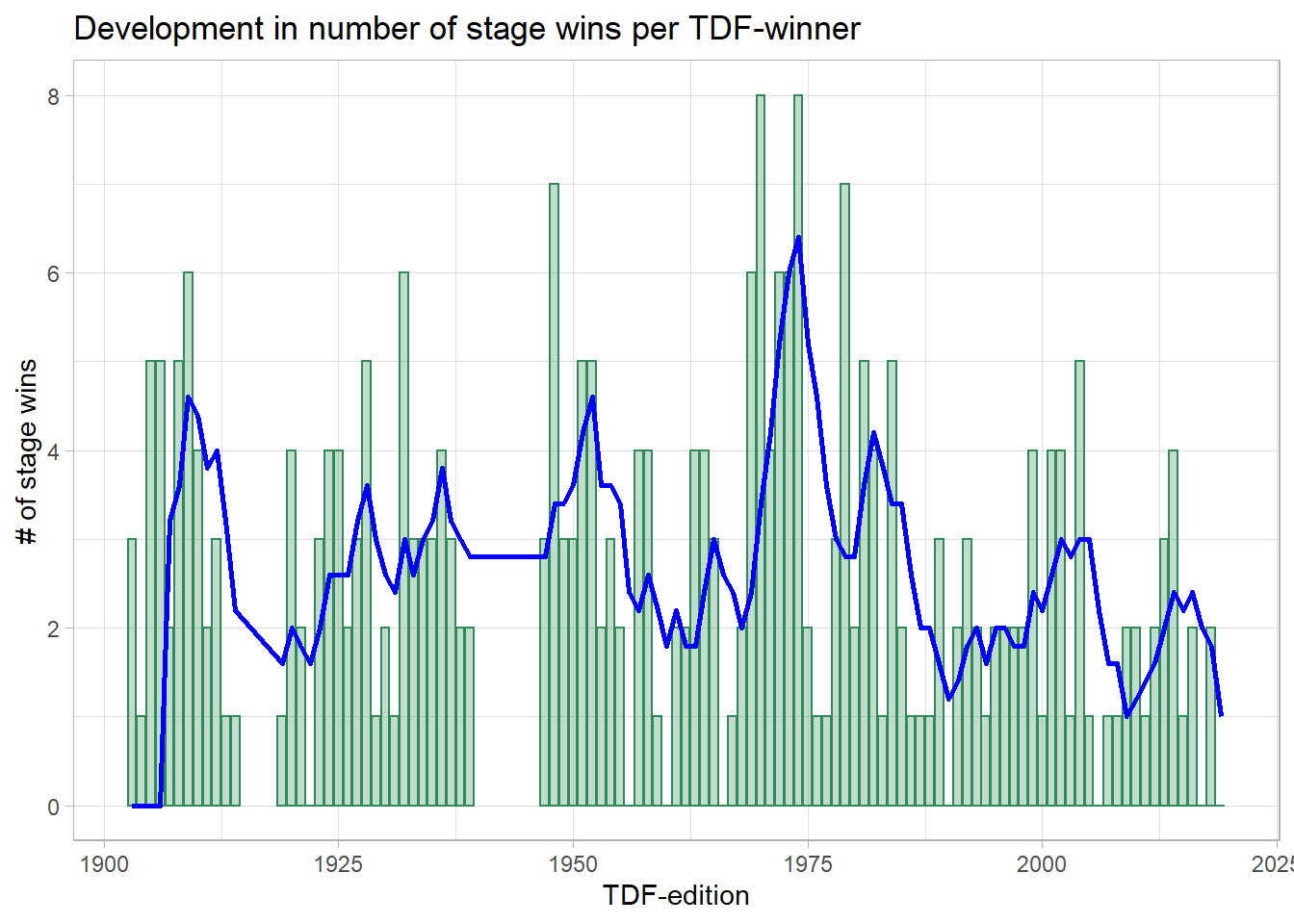
Some observations:
- The gaps represent the world wars, where TDF had to be cancelled. This year’s edition is the first edition since WW2 that has been postponed or cancelled.
- There’s a large peak in number of stage wins around 1970-1975. This is due to the dominance of arguably the best cyclist of all time, Eddy Merckx, who won the TDF 5 times with no less than 34 stage wins.
- There’s a weak trend that the winners nowadays pick up fewer stage wins, but I have to say that the effect is lower than I expected (particularly if you remove the “Eddy Merckx”-effect)
Average speed
Let’s look at the development in speed over the years.
winners %>%
  mutate(speed = distance / time_overall) %>%
  ggplot(aes(x = year(start_date), y = speed)) +
  geom_point() +
  geom_smooth(span = 0.2, color = "seagreen4")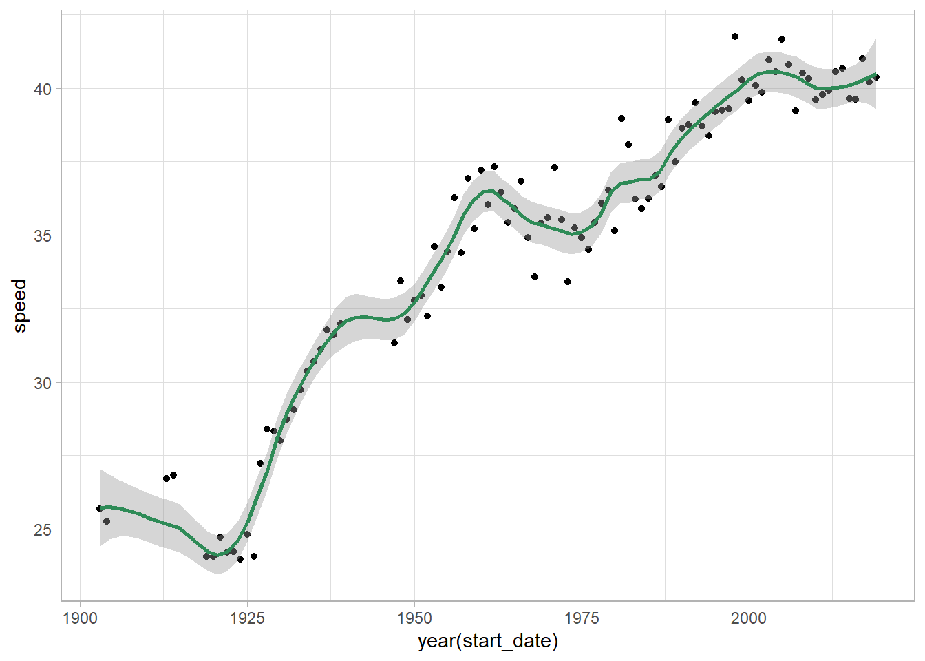
As we can see, the average speed has increased from around 25 kph at the start (a pace most amateur cyclists can hold today - but probably not with 1900-quality equipment) to 40 kph the last few years. We do see, however, that the pace fell slightly after around 2003, which incidently the time EPO test was developed.
Let’s zoom in on the last few years to get a closer look.
library(ggforce)
desc_1990 <- "EPO-use is widespread in the peloton and no tests exists"
desc_2000 <- "The first tests for EPO are introduced"
desc_2008 <- "Riders are also monitored using the blood passport"

winners %>%
  mutate(speed = distance / time_overall,
         year = year(start_date)) %>%
  ggplot(aes(x = year, y = speed)) +
  geom_mark_ellipse(aes(filter = year >= 1990 & year < 2000,
                        description = desc_1990),
                    label.fontsize = 8) +
  geom_mark_ellipse(aes(filter = year >= 2000 & year < 2008,
                        description = desc_2000),
                    label.fontsize = 8) +
  geom_mark_ellipse(aes(filter = year >= 2008,
                        description = desc_2008),
                    label.fontsize = 8) +
  geom_point() +
  geom_smooth(span = 0.15, color = "seagreen4") +
  coord_cartesian(xlim = c(1985, 2020), ylim = c(33, 42)) +
  labs(title = "Development in speed (KPH) for TDF-winners")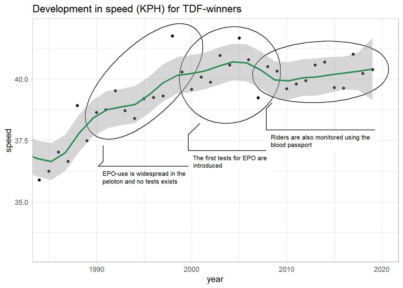
Looking at the speed alone, in connection with important historical events in anti-doping, it does seem like the increase in speed flattens out or drops each time a new “weapon” in the fight against doping is introduced.
Of course, such an analysis is very simplistic, and to get the whole picture one also needs to take into account altitude meters ascended, road quality, equipment, race tactics and so on.
Stage winners
Let’s look at the number of stage wins per rider, ordered by category.
# Clean up - mix between lower and higher letters
stages <- stages %>%
  mutate(Type = str_to_lower(Type))

stages %>%
  group_by(Winner) %>%
  mutate(total_stage_wins = n()) %>%
  ungroup() %>%
  mutate(winner_lmp = fct_lump(Winner, 30)) %>%
  count(winner_lmp, Type, total_stage_wins, sort = TRUE) %>%
  filter(winner_lmp != "Other") %>%
  ggplot(aes(x = fct_reorder(winner_lmp, total_stage_wins), y = n, fill = Type)) +
  geom_col() +
  coord_flip() +
  scale_fill_viridis_d() +
  labs(x = NULL)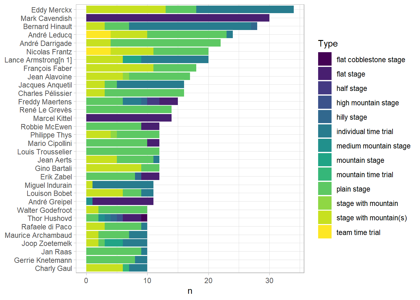
Note that the top riders are a mix between pure specialists, such as the sprinters like Mark Cavendish and Marcel Kittel, and more versatile riders.
So that leads to the question - who is the most versatile TDF-rider? An easy metric would be to check which rider has recorded the largest number of different stage wins.
stages %>%
  group_by(Winner) %>%
  summarise(total_stage_wins = n(),
         different_stage_wins = n_distinct(Type)) %>%
  arrange(-different_stage_wins, - total_stage_wins) %>%
  slice(1:10) %>%
knitr::kable()| Winner | total_stage_wins | different_stage_wins |
|---|---|---|
| Thor Hushovd | 10 | 7 |
| Freddy Maertens | 15 | 5 |
| Sylvère Maes | 9 | 5 |
| Bernard Hinault | 28 | 4 |
| André Leducq | 24 | 4 |
| Joop Zoetemelk | 10 | 4 |
| Antonin Magne | 9 | 4 |
| Bernard Thévenet | 9 | 4 |
| Ferdinand Kübler | 8 | 4 |
| Chris Froome | 7 | 4 |
The Norwegian rider Thor Hushovd ends up on the top here - with a mix of time trials, flat stages, medium mountain stages, hilly stages, a cobbled stage and even a high mountain stage (“The Miracle in Lourdes”, as we say in Norway), he comes out on top with no less than 7 different stage wins:
stages %>%
  filter(Winner == "Thor Hushovd") %>%
  select(-Winner, - Winner_Country) %>%
knitr::kable()| Stage | Date | Distance | Origin | Destination | Type |
|---|---|---|---|---|---|
| 13 | 2011-07-15 | 152.5 | Pau | Lourdes | high mountain stage |
| 16 | 2011-07-19 | 162.5 | Saint-Paul-Trois-Châteaux | Gap | medium mountain stage |
| 3 | 2010-07-06 | 213.0 | Wanze | Arenberg Porte du Hainaut | flat cobblestone stage |
| 6 | 2009-07-09 | 181.5 | Girona | Barcelona | flat stage |
| 2 | 2008-07-06 | 164.5 | Auray | Saint-Brieuc | flat stage |
| 4 | 2007-07-11 | 193.0 | Villers-Cotterêts | Joigny | plain stage |
| P | 2006-07-01 | 7.1 | Strasbourg | Strasbourg | individual time trial |
| 20 | 2006-07-23 | 154.5 | Antony/Parc de Sceaux | Paris | flat stage |
| 8 | 2004-07-11 | 168.0 | Lamballe | Quimper | plain stage |
| 18 | 2002-07-26 | 176.5 | Cluses | Bourg-en-Bresse | hilly stage |
This comparison is definitely not completely fair, though - there appears to be a larger number of stage types in the later years, which is probably not due to more varied courses, but more detailed registrations of stage types. Moreover, versatility should be measured by placements, not just by victories. Nonetheless, it is an interesting statistic.
We can also use the positions-dataset to get a closer look at the placements of all riders per stage. Let’s have a closer look at Hushovd’s career using a heatmap.
p <- rankings %>%
  filter(rider == "Hushovd Thor") %>%
  mutate(rank = as.numeric(rank),
         stage = factor(as.numeric(str_remove(stage_results_id, "stage-"))),
         year = factor(year)) %>%
  ggplot(aes(x = year, y = stage, fill = rank)) +
  geom_tile() +
  scale_fill_viridis_c() +
  geom_text(aes(label = rank), size = 2, color = "white") +
  labs(x = "Year", y = "Stage number", title = "Thor Hushovd's TDF-career in a heatmap")

plotly::ggplotly(p, tooltip = c("y", "x", "fill"))
That’s it for now, but there is definitely more to explore in this dataset!