Little is more frustrating then writing code that is mind-numbingly slow, but you have no idea how to fix it, so you just end up waiting for several minutes each time your code runs. Now, this isn’t always a huge problem (maybe you needed a break anyway). However, for code in production, speed is absolutely essential.
In this blog post, I will go over 5 tips that may help you speed your R-code.
1) Bench::mark and profile your code!
My first tip will not directly speed up your code, but will help you identify improvements.
Start by profiling your code. In Rstudio, this can be done by selecting the code of interest and pressing CTRL + Shift + Alt + P. This will bring up statistics on how fast each part of your code is, and might help you identify bottlenecks.
When the bottleneck has been identified, test it against alternatives using bench::mark. Personally I prefer this package to the alternatives as it also makes sure the results of your tests are identical, unless you specify check = FALSE.
2) Avoid slow base-R functions
Some of the base-R functions are excruciatingly slow and should be avoided for large data sets.
I will go through a few of them here.
Avoid “ifelse”
df <- tibble(
  x = rnorm(30000000),
  y = rnorm(30000000)
)

bench::mark(
  df$z <- ifelse(df$x > df$y, 1, 0),
  df$z <- if_else(df$x > df$y, 1, 0),
  df$z <- case_when(df$x > df$y ~ 1,
                TRUE ~ 0)
)
## # A tibble: 3 x 10
## expression min mean median max `itr/sec` mem_alloc n_gc
## <chr> <bch:tm> <bch:tm> <bch:tm> <bch:tm> <dbl> <bch:byt> <dbl>
## 1 df$z <- i~ 2.21s 2.21s 2.21s 2.21s 0.453 3.46GB 7
## 2 df$z <- i~ 979.83ms 979.83ms 979.83ms 979.83ms 1.02 2.01GB 3
## 3 df$z <- c~ 1.9s 1.9s 1.9s 1.9s 0.528 3.02GB 5
## # ... with 2 more variables: n_itr <int>, total_time <bch:tm>As we can see, dplyr::if_else is the best option here. However, all the functions are actually quite slow, so as a slightly less readable alternative, you can make the variable in a different manner: first, create a vector with one of the possible values, then filter and replace the rest.
DT <- as.data.table(df)

bench::mark({
  # Using base-R
  df$z <- 0
  df$z[df$x > df$y] <- 1
},
{
  # Using data.table
  DT[, z := 0]
  DT[x > y, z := 1]
},
check = FALSE)
## # A tibble: 2 x 10
## expression min mean median max `itr/sec` mem_alloc n_gc n_itr
## <chr> <bch> <bch> <bch:> <bch> <dbl> <bch:byt> <dbl> <int>
## 1 {... 319ms 319ms 319ms 319ms 3.13 744MB 1 1
## 2 {... 479ms 482ms 482ms 485ms 2.07 402MB 0 2
## # ... with 1 more variable: total_time <bch:tm>Here we see that both these options are far superior to ifelse/if_else/case_when in terms of both speed and memory usage. In the end, a variation using exclusively base-R ended up as the fastest (while data.table is a clear winner in terms of memory usage, probably due to avoiding copies).
Avoid as.Date
When converting a variable to a date it might be tempting to use as.Date. If you are working with big data, this is a big mistake! ymd or as_date from lubridate are far better options. We will compare the speed of the different variations using bench::press, which allows us to do the tests for varying sizes of the data.
generate_dates <- function(n) {
    as.character(sample(seq(
    ymd("1999-01-01"), ymd("2018-01-01"), by = "day"
    ), n, replace = TRUE))
}


results <- bench::press(
  n = c(500000, 1000000, 3000000),
  {
   dates <- generate_dates(n)
    bench::mark(
      min_iterations = 3,
      lubridate::ymd(dates),
      lubridate::as_date(dates),
      as.Date(dates)
    )
  }
)

autoplot(results)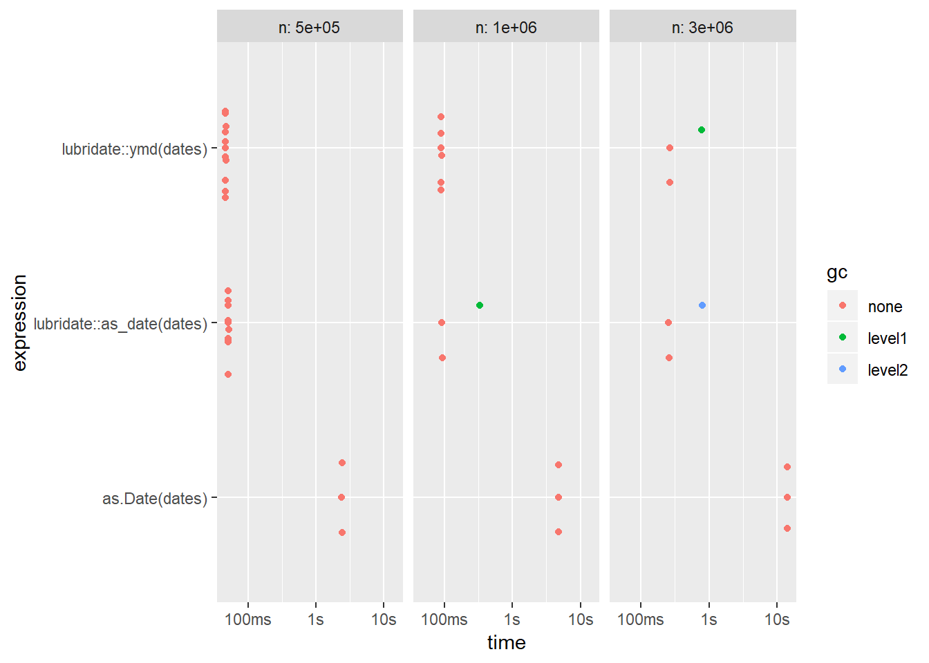
The two lubridate variations seem to be equal, but as we can tell, as.Date is a lot slower and we’re just on 5 million rows here. With several million rows, as.Date quickly becomes completely unusable.
Other base functions to avoid
I recommend to avoid the following base functions due to speed issues:
- read.csv (use readr::read_csv or data.table::fread)
- aggregate (use dplyr:: group_by + summarise or data.tables [i, j, by]-syntax)
- merge (use dplyr::left_join or data.table::merge)
3) Believe in The Matrix
A lot of people who start up in R seems to exclusively use data-frames, and completely avoid the other data structures, such as matrices or even lists.
Several times, I have seen people do matrix-like operations on data-frames that could and should have been converted to a matrix. Of course, matrices cannot always be used, as they have very strict requirements (all columns must be of the same type).
Let’s look at a trivial example, where we pick a few rows and add them together.
m <- as.matrix(df)

bench::mark(
  m[1,] + m[2,] + m[3,],
  df[1,] + df[2,] + df[3,],
  check = FALSE,
  relative = TRUE,
  min_iterations = 5
)
## # A tibble: 2 x 10
## expression min mean median max `itr/sec` mem_alloc n_gc n_itr
## <chr> <dbl> <dbl> <dbl> <dbl> <dbl> <dbl> <dbl> <dbl>
## 1 m[1, ] + ~ 1 1 1 1 314. NaN NaN 11.3
## 2 df[1, ] +~ 359. 314. 276. 30.9 1 Inf NaN 1
## # ... with 1 more variable: total_time <dbl>For this simple example, using a matrix resulted in a ~250 times speed increase on average!
“Why, oh why, didn’t I take the blue pill?”
The Matrix (1999).
4) Use The Database, Luke
Here’s a quick tip which could improve your speed if you are working with data from a database.
Simply replace your calls to the RODBC-package with the significantly faster combination of DBI + odbc. In my opinion, it is not only faster, but has better syntax too.
Another tip is to filter and select the data you want before collecting it to your local memory. This can either be done by writing the SQL-code yourself, or by using the excellent dbplyr-functionality (dbplyr translates your R-code to SQL and executes the commands directly in the database).
Here is an example of what this could look like.
conn <- dbConnect(odbc(),
                 pwd = password,
                 uid = user,
                 server = server
                 )

# Make a pointer to the database, filter, select and THEN collect the data
df <- tbl(conn) %>%
  filter(age > 30) %>%
  select(age, gender, nationality) %>%
  collect()
“For my ally is The Database, and a powerful ally it is.”
— Yoda, Star Wars (note: quote might be slightly modified)
5) Use data.table for large datasets
Are you working with data sets larger than a few gigabytes and still sticking with dplyr?
While dplyr is an excellent package with beautiful syntax, it is not optimized for big data. “data.table”, on the other hand, is made to work well with huge data sets. The drawback, in my opinion, is that the syntax is not as pretty and it includes some dangerous features which could cause a lot of frustration for beginners (such as updating by reference).
To illustrate, I will compare two simple grouped calculations using dplyr and data.table respectively, for 10 million and 100 million rows.
set.seed(1)

simulate_data <- function(n) {
  df <- tibble(x = rnorm(n),
               y = rnorm(n),
               z1 = sample(1:8, n, replace = T),
               z2 = sample(1:8, n, replace = T))

}


results <- bench::press(
  rows = c(10000000, 100000000),
  {
    df <- simulate_data(rows)
    DT <- as.data.table(simulate_data(rows))
    bench::mark(
      min_iterations = 5,
      df %>% group_by(z1, z2) %>% summarise(sum_x = sum(x), sum_y = sum(y)),
      DT[, .(sum_x = sum(x), sum_y = sum(y)), by = .(z1, z2)],
      check = FALSE
    )
  }
)

autoplot(results) + scale_x_discrete(labels = c("dplyr", "data.table"))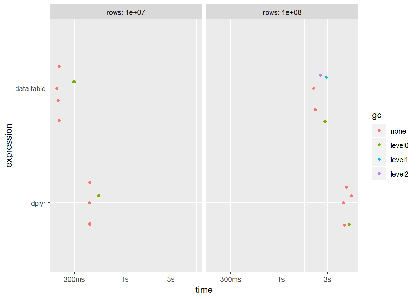
The results show that data.table is faster, but the difference is actually a lot smaller than I expected for this particular example.
For a more comprehensive comparison, see H20’s speed test where they compare data.table to dplyr, pandas and more: https://h2oai.github.io/db-benchmark/.
In a later blog post, I will also explore how you can use parallelization with the excellent “future”-package to improve speed.